UNet算法思想

UNet简介

论文来自：[1505.04597] U-Net: Convolutional Networks for Biomedical Image Segmentation
特点：
- 高效利用数据增强：使用弹性形变(elastic deformations)扩充数据集，少量数据图像便可训练
- 提供新型网络结构：使用收缩路径(contracting path)捕获信息和对称扩展路径(symmetric expanding path)精确定位，跳跃连接（Skip Connections）将两者结合的全卷积神经网络
- 提供新型训练策略：使用重叠瓦片策略(Overlap-tile strategy)，使用加权损失函数，分隔触碰细胞的背景标签在损失函数中获取较大的权重
适用范围：生物医学图像处理，属于分类任务，但是特征与标签之间是1：n的关系，在图像的不同区域，标签不同
创新点(对比滑动窗口)：
- 滑动窗口要对图像进行分割成不同的补丁(patch)图像，每个补丁对应一个标签，滑动窗口的补丁图像的数量大于原始图像的数量，且要对每个补丁图像进行训练，效率低下
- 如果补丁图像较大，定位精度不够，且需要更多的池化层，如果补丁图像太小，补丁图像与周围图像关系不太明显

UNet网络结构

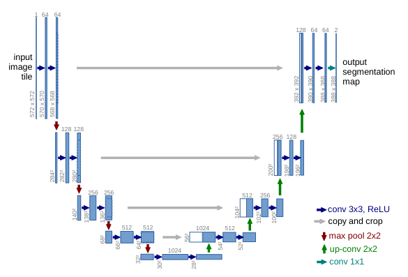
特点：
1. 网络只使用卷积层，在U型结构的一侧使用池化层，对应的另一侧使用上采样层
2. 剪切收缩路径的高分辨率特征并与扩展路径特征合并，如图上蓝白方框
3. 使用收缩路径和扩展路径，收缩路径在左侧，扩展路径在右侧，形成“U”型结构

代码实现：

class UNet(nn.Module):
    def __init__(self):
        super(UNet, self).__init__()
        # 卷积计算公式: output = (input - kernel_size + 2*padding) / stride + 1
        # input (1, 572, 572)
        self.layer1 = nn.Sequential(
            nn.Conv2d(1, 64, 3, 1, 0),  # output (64, 570, 570)
            nn.ReLU(),
            nn.Conv2d(64, 64, 3, 1, 0),  # output (64, 568, 568)
            nn.ReLU()
        )
        self.layer2 = nn.Sequential(
            nn.MaxPool2d(2),  # output (64, 284, 284)
            nn.Conv2d(64, 128, 3, 1, 0),  # output (128, 282, 282)
            nn.ReLU(),
            nn.Conv2d(128, 128, 3, 1, 0),  # output (128, 280, 280)
            nn.ReLU()
        )
        self.layer3 = nn.Sequential(
            nn.MaxPool2d(2),  # output (128, 140, 140)
            nn.Conv2d(128, 256, 3, 1, 0),  # output (128, 138, 138)
            nn.ReLU(),
            nn.Conv2d(256, 256, 3, 1, 0),  # output (256, 136, 136)
            nn.ReLU()
        )
        self.layer4 = nn.Sequential(
            nn.MaxPool2d(2),  # output (256, 68, 68)
            nn.Conv2d(256, 512, 3, 1, 0),  # output (512, 66, 66)
            nn.ReLU(),
            nn.Conv2d(512, 512, 3, 1, 0),  # output (512, 64, 64)
            nn.ReLU()
        )
        self.layer5 = nn.Sequential(
            nn.MaxPool2d(2),  # output (512, 32, 32)
            nn.Conv2d(512, 1024, 3, 1, 0),  # output (1024, 30, 30)
            nn.ReLU(),
            nn.Conv2d(1024, 1024, 3, 1, 0),  # output (1024, 28, 28)
            nn.ReLU(),
            nn.ConvTranspose2d(1024, 512, 2, 2, 0)  # output (512, 56, 56)
        )
        # 上采样计算公式：output = stride * (input - 1) + kernel_size - 2*padding + (input + 2 padding - kernel) mod stride
        # input (1024, 56, 56)
        self.layer6 = nn.Sequential(
            nn.Conv2d(1024, 512, 3, 1, 0),
            nn.ReLU(),
            nn.Conv2d(512, 512, 3, 1, 0),
            nn.ReLU(),
            nn.ConvTranspose2d(512, 256, 2, 2, 0)   # output (512, 104, 104)
        )
        self.layer7 = nn.Sequential(
            nn.Conv2d(512, 256, 3, 1, 0),   # output (256, 102, 102)
            nn.ReLU(),
            nn.Conv2d(256, 256, 3, 1, 0),   # output (256, 100, 100)
            nn.ReLU(),
            nn.ConvTranspose2d(256, 128, 2, 2, 0)   # output (256, 200, 200)
        )
        self.layer8 = nn.Sequential(
            nn.Conv2d(256, 128, 3, 1, 0),   # output (128, 198, 198)
            nn.ReLU(),
            nn.Conv2d(128, 128, 3, 1, 0),   # output (128, 196, 196)
            nn.ReLU(),
            nn.ConvTranspose2d(128, 64, 2, 2, 0)    # output (128, 392, 392)
        )
        self.layer9 = nn.Sequential(
            nn.Conv2d(128, 64, 3, 1, 0),    # output (64, 390, 390)
            nn.ReLU(),
            nn.Conv2d(64, 64, 3, 1, 0),     # output (64, 388, 388)
            nn.ReLU(),
            nn.Conv2d(64, 2, 1, 1, 0)
        )
    # 前行传播
    def forward(self, x):
        skip1 = self.layer1(x)
        skip2 = self.layer2(skip1)
        skip3 = self.layer3(skip2)
        skip4 = self.layer4(skip3)

        output = self.layer5(skip4)
        # 剪切
        skip1 = skip1[:, 87: 479, 87: 479]
        skip2 = skip2[:, 39: 239, 39: 239]
        skip3 = skip3[:, 15: 119, 15: 119]
        skip4 = skip4[:, 3: 59, 3: 59]
        # 合并
        output = self.layer6(torch.cat((skip4, output)))
        output = self.layer7(torch.cat((skip3, output)))
        output = self.layer8(torch.cat((skip2, output)))
        output = self.layer9(torch.cat((skip1, output)))
        return output

模型参数量：31030658(float64)
模型输入输出：输入为(1, 572, 572)的灰度图像特征，输出为(C, 388, 388)，其中C为类别数目，本例为C=2

训练过程

优化器：随机梯度下降(stochastic gradient desecnt)，采用大动量(momentum=0.99)之前训练的结构将大幅决定本轮优化方向
batch_size：一个图像，输入大图像而不是大批量
损失函数：对逐个像素使用soft-max函数，对整体特征图像采用交叉熵损失函数

交叉熵损失函数

应用：本论文的损失函数为像素级的交叉熵损失(Pixel-wise Cross-Entropy Loss),引入了一个创新的加权损失机制，用于突出细胞边界的重要性
公式：$$L = -\sum_{x \in \Omega}\sum_{c=1}^Cy_c(x)log(p_c(x))$$其中$\Omega$为像素全集，c为类别数量

soft-max函数

应用：对每个像素点应用
公式：$$p_k(x) = exp(a_k(x))/(\sum_{k=1}^K exp(a_k(x)))$$其中k表示的是分类，$p_k(x)$是最大近似函数，$a_k(x)$是在像素位置x的特征通道k的激活函数

加权交叉熵损失函数

特点：加权损失函数，为边界像素分配更高的权重
公式：$$w(x) = w_c(x) + w_0*exp(-\frac{(d_1(x) + d_2(x))^2}{2})$$其中$w_c$是权重地图平衡类别频率，$d_1$是到最近的细胞边界的距离，$d_2$是到第二近的细胞的距离，实验得$w_0 = 10 \quad \sigma = 5$

数据增广

几何变换

类型：
**平移(Translation)**：随机移动图像，模拟细胞在图像中的不同位置
**旋转(Rotation)**：随机旋转图像，增加对角度变化的鲁棒性
**缩放(Scaling)**：轻微缩放图像，模拟显微镜成像的不同放大倍率
原理：平移和旋转不变性(shift and rotation invariance)
注意：掩码与原图像要做相同的图像变换

弹性形变

定义：模拟生物组织的非刚性形变(如细胞的拉伸、扭曲)，在生物医学图像中尤为重要，因为细胞形状和排列高度可变
步骤：
1. 在图像上定义一个粗糙网格(论文提到 3x3 网格，覆盖整个图像)
2. 为每个网格点生成随机位移向量(Random Displacement Vectors)，基于高斯分布(“displacement vectors sampled from a Gaussian distribution”)
3. 使用双线性插值将位移场平滑应用到整个图像，生成变形后的图像。
4. 对分割掩码应用相同的位移场，确保一致性。

实例代码

# 导入库函数  
import torch  
import matplotlib.pyplot as plt  
import torch.nn as nn  
from torch.utils.data import DataLoader, Dataset  
from torchvision import transforms  
import random  
import numpy as np  
import os  
import torch.optim as optim  
  
  
# utils 工具  
  
# 随机种子函数 方便复现  
def seed_everything(seed):  
    torch.manual_seed(seed)  
    torch.cuda.manual_seed(seed)  
    torch.cuda.manual_seed_all(seed)  
    torch.backends.cudnn.benchmark = False  
    torch.backends.cudnn.deterministic = True  
    random.seed(seed)  
    np.random.seed(seed)  
    os.environ['PYTHONHASHSEED'] = str(seed)  
  
  
# 展示模型  
def model_structure(model):  
    blank = ' '  
    print('-' * 90)  
    print('|' + ' ' * 11 + 'weight name' + ' ' * 10 + '|' \  
          + ' ' * 15 + 'weight shape' + ' ' * 15 + '|' \  
          + ' ' * 3 + 'number' + ' ' * 3 + '|')  
    print('-' * 90)  
    num_para = 0  
    type_size = 1  # 如果是浮点数就是4  
  
    for index, (key, w_variable) in enumerate(model.named_parameters()):  
        if len(key) <= 30:  
            key = key + (30 - len(key)) * blank  
        shape = str(w_variable.shape)  
        if len(shape) <= 40:  
            shape = shape + (40 - len(shape)) * blank  
        each_para = 1  
        for k in w_variable.shape:  
            each_para *= k  
        num_para += each_para  
        str_num = str(each_para)  
        if len(str_num) <= 10:  
            str_num = str_num + (10 - len(str_num)) * blank  
  
        print('| {} | {} | {} |'.format(key, shape, str_num))  
    print('-' * 90)  
    print('The total number of parameters: ' + str(num_para))  
    print('The parameters of Model {}: {:4f}M'.format(model._get_name(), num_para * type_size / 1000 / 1000))  
    print('-' * 90)  
  
  
# 变换图像  
transform = transforms.Compose([  
    transforms.ToPILImage(),  # img (572, 572, 1) -> (1, 572, 572)  
    transforms.ToTensor()  # 转化为 Tensor类型  
])  
  
  
# 计算权重图  
def compute_weight_map():  
    return torch.tensor([1])  
  
  
# super 超参  
batch_size = 1  
epochs = 40  
  
  
# step 1: 导入数据集  
# 导入数据集，有数据集之后在写 记得用transform将图像变换为Tensor  
class BioImageDataset(Dataset):  
    def __init__(self, file_path, mode):  
        pass  
  
    def __getitem__(self, idx):  
        pass  
  
    def __len__(self):  
        pass  
  
  
train_file = "<此处填入数据集路径>"  
test_file = "<此处填入测试集路径>"  
  
train_dataset = BioImageDataset(train_file, mode="train")  
val_dataset = BioImageDataset(train_file, mode="val")  
test_dataset = BioImageDataset(test_file, mode="test")  
  
# 打乱数据集  
train_loader = DataLoader(train_dataset, batch_size=batch_size, shuffle=True)  
val_loader = DataLoader(val_dataset, batch_size=batch_size, shuffle=True)  
# 用于预测不打乱  
test_dataset = DataLoader(test_dataset, batch_size=1, shuffle=False)  
  
  
# step 2: 定义模型  
class UNet(nn.Module):  
    def __init__(self):  
        super(UNet, self).__init__()  
        # 卷积计算公式: output = (input - kernel_size + 2*padding) / stride + 1  
        # input (1, 572, 572)        self.layer1 = nn.Sequential(  
            nn.Conv2d(1, 64, 3, 1, 0),  # output (64, 570, 570)  
            nn.ReLU(),  
            nn.Conv2d(64, 64, 3, 1, 0),  # output (64, 568, 568)  
            nn.ReLU()  
        )  
        self.layer2 = nn.Sequential(  
            nn.MaxPool2d(2),  # output (64, 284, 284)  
            nn.Conv2d(64, 128, 3, 1, 0),  # output (128, 282, 282)  
            nn.ReLU(),  
            nn.Conv2d(128, 128, 3, 1, 0),  # output (128, 280, 280)  
            nn.ReLU()  
        )  
        self.layer3 = nn.Sequential(  
            nn.MaxPool2d(2),  # output (128, 140, 140)  
            nn.Conv2d(128, 256, 3, 1, 0),  # output (128, 138, 138)  
            nn.ReLU(),  
            nn.Conv2d(256, 256, 3, 1, 0),  # output (256, 136, 136)  
            nn.ReLU()  
        )  
        self.layer4 = nn.Sequential(  
            nn.MaxPool2d(2),  # output (256, 68, 68)  
            nn.Conv2d(256, 512, 3, 1, 0),  # output (512, 66, 66)  
            nn.ReLU(),  
            nn.Conv2d(512, 512, 3, 1, 0),  # output (512, 64, 64)  
            nn.ReLU()  
        )  
        self.layer5 = nn.Sequential(  
            nn.MaxPool2d(2),  # output (512, 32, 32)  
            nn.Conv2d(512, 1024, 3, 1, 0),  # output (1024, 30, 30)  
            nn.ReLU(),  
            nn.Conv2d(1024, 1024, 3, 1, 0),  # output (1024, 28, 28)  
            nn.ReLU(),  
            nn.ConvTranspose2d(1024, 512, 2, 2, 0)  # output (512, 56, 56)  
        )  
        # 上采样计算公式：output = stride * (input - 1) + kernel_size - 2*padding + (input + 2 padding - kernel) mod stride  
        # input (1024, 56, 56)        self.layer6 = nn.Sequential(  
            nn.Conv2d(1024, 512, 3, 1, 0),  
            nn.ReLU(),  
            nn.Conv2d(512, 512, 3, 1, 0),  
            nn.ReLU(),  
            nn.ConvTranspose2d(512, 256, 2, 2, 0)  # output (512, 104, 104)  
        )  
        self.layer7 = nn.Sequential(  
            nn.Conv2d(512, 256, 3, 1, 0),  # output (256, 102, 102)  
            nn.ReLU(),  
            nn.Conv2d(256, 256, 3, 1, 0),  # output (256, 100, 100)  
            nn.ReLU(),  
            nn.ConvTranspose2d(256, 128, 2, 2, 0)  # output (256, 200, 200)  
        )  
        self.layer8 = nn.Sequential(  
            nn.Conv2d(256, 128, 3, 1, 0),  # output (128, 198, 198)  
            nn.ReLU(),  
            nn.Conv2d(128, 128, 3, 1, 0),  # output (128, 196, 196)  
            nn.ReLU(),  
            nn.ConvTranspose2d(128, 64, 2, 2, 0)  # output (128, 392, 392)  
        )  
        self.layer9 = nn.Sequential(  
            nn.Conv2d(128, 64, 3, 1, 0),  # output (64, 390, 390)  
            nn.ReLU(),  
            nn.Conv2d(64, 64, 3, 1, 0),  # output (64, 388, 388)  
            nn.ReLU(),  
            nn.Conv2d(64, 2, 1, 1, 0)  
        )  
  
    # 前行传播  
    def forward(self, x):  
        skip1 = self.layer1(x)  
        skip2 = self.layer2(skip1)  
        skip3 = self.layer3(skip2)  
        skip4 = self.layer4(skip3)  
  
        output = self.layer5(skip4)  
        # 剪切  
        skip1 = skip1[:, 87: 479, 87: 479]  
        skip2 = skip2[:, 39: 239, 39: 239]  
        skip3 = skip3[:, 15: 119, 15: 119]  
        skip4 = skip4[:, 3: 59, 3: 59]  
        # 合并  
        output = self.layer6(torch.cat((skip4, output)))  
        output = self.layer7(torch.cat((skip3, output)))  
        output = self.layer8(torch.cat((skip2, output)))  
        output = self.layer9(torch.cat((skip1, output)))  
        return output  
  
  
# step 3: 模型训练  
  
device = "cuda" if torch.cuda.is_available() else "cpu"  
model = UNet().to(device)  
optimizer = optim.SGD(model.parameters(), lr=0.01, momentum=0.99)  
loss = nn.BCEWithLogitsLoss()  
  
  
def train(model, optim, epochs):  
    for epoch in range(epochs):  
        model.train()  
        # 记录损失值  
        total_loss = 0  
        for image, mask in train_loader:  
            image = image.to(device)  
            mask = mask.to(device)  
            weight = compute_weight_map().to(device)  
            output = model(image)  
            Loss = loss(output, mask, weight=weight)  
            optim.zero_grad()  
            Loss.backward()  
            optim.step()  
            total_loss += Loss.item()  
        print(f'Epoch [{epoch+1}/40], Loss: {total_loss / len(train_loader):.4f}')  
  
  
# step 4: 模型评估  
  
# step 5: 模型预测

UNet++算法思想

UNet++简介

论文来自：[1807.10165] UNet++: A Nested U-Net Architecture for Medical Image Segmentation
特点：
- 新型网络结构：深度监督编码解码网络(deeply-surpervised encoder-decoder Network)，其中编码器，解码器通过一系列嵌套的密集的跳跃步骤，重新设计跳跃路径，减少编码器和解码器子网络特征图之间的语义差距
适用范围：生物医学领域的标注数据非常少，分割需要像素级预测
创新点：
- 特征融合不足：跳跃连接直接拼接编码器和解码器的特征图，但缺乏中间层次的特征融合，可能导致语义差距（Semantic Gap）
- 单一路径限制：U-Net 的单一编码-解码路径可能无法充分捕获多尺度特征，尤其在复杂组织结构（如肿瘤）分割中

网络结构

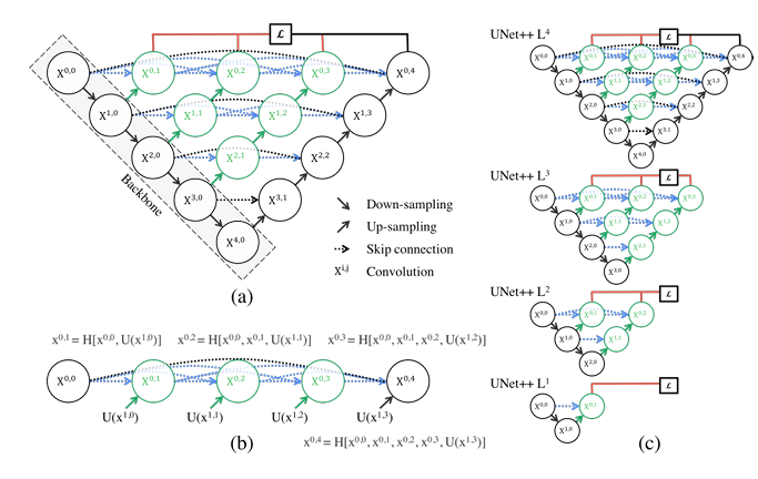
特点：
1. 新型网络结构：引入密集跳跃连接（Dense Skip Connections），形成嵌套的子网络，增强多尺度特征融合
2. **深度监督(Deep Supervision)**：
3. **剪枝优化(Pruning)**：

实例代码：

# 双卷积块（Double Convolution）
class DoubleConv(nn.Module):
    def __init__(self, in_channels, out_channels):
        super(DoubleConv, self).__init__()
        self.double_conv = nn.Sequential(
            nn.Conv2d(in_channels, out_channels, kernel_size=3, padding=1, bias=False),
            nn.BatchNorm2d(out_channels),  # 论文未明确使用 BN，现代实现常添加
            nn.ReLU(inplace=True),
            nn.Conv2d(out_channels, out_channels, kernel_size=3, padding=1, bias=False),
            nn.BatchNorm2d(out_channels),
            nn.ReLU(inplace=True)
        )
    
    def forward(self, x):
        return self.double_conv(x)

# 下采样模块（Downsampling）
class Down(nn.Module):
    def __init__(self, in_channels, out_channels):
        super(Down, self).__init__()
        self.maxpool_conv = nn.Sequential(
            nn.MaxPool2d(kernel_size=2, stride=2),
            DoubleConv(in_channels, out_channels)
        )
    
    def forward(self, x):
        return self.maxpool_conv(x)

# 上采样模块（Upsampling）
class Up(nn.Module):
    def __init__(self, in_channels, out_channels):
        super(Up, self).__init__()
        self.up = nn.ConvTranspose2d(in_channels, in_channels // 2, kernel_size=2, stride=2)
        self.conv = DoubleConv(in_channels, out_channels)  # 输入通道数为拼接后的通道数
    
    def forward(self, x1, skip_connections):
        x1 = self.up(x1)
        # 调整尺寸以匹配 skip_connections
        diffY = skip_connections[0].size()[2] - x1.size()[2]
        diffX = skip_connections[0].size()[3] - x1.size()[3]
        x1 = F.pad(x1, (diffX // 2, diffX - diffX // 2, diffY // 2, diffY - diffY // 2))
        # 拼接所有 skip_connections
        x = torch.cat([x1] + skip_connections, dim=1)
        return self.conv(x)

# UNet++ 模型
class UNetPlusPlus(nn.Module):
    def __init__(self, n_channels, n_classes, deep_supervision=True, level=4):
        super(UNetPlusPlus, self).__init__()
        self.deep_supervision = deep_supervision
        self.level = level
        
        # 编码器
        self.inc = DoubleConv(n_channels, 64)
        self.down1 = Down(64, 128)
        self.down2 = Down(128, 256)
        self.down3 = Down(256, 512)
        self.down4 = Down(512, 1024)
        
        # 解码器节点（X^{i,j}）
        self.up1 = {}  # 存储上采样节点
        self.outc = {}  # 存储输出卷积
        
        # 初始化解码器节点
        for i in range(4):  # 对应 4 个下采样级别
            for j in range(1, self.level + 1 - i):  # 嵌套路径数随级别减少
                if i == 0:  # 顶层输出节点
                    self.up1[f'x{i}_{j}'] = Up(2 ** (6 - i) * 2 ** j, 2 ** (6 - i))
                    self.outc[f'x{i}_{j}'] = nn.Conv2d(2 ** (6 - i), n_classes, kernel_size=1)
                else:
                    self.up1[f'x{i}_{j}'] = Up(2 ** (7 - i) * 2 ** (j - 1), 2 ** (6 - i))
        
        # 将字典转换为 nn.ModuleDict
        self.up1 = nn.ModuleDict(self.up1)
        self.outc = nn.ModuleDict(self.outc)
    
    def forward(self, x):
        # 编码器路径
        x0_0 = self.inc(x)        # 64, H, W
        x1_0 = self.down1(x0_0)   # 128, H/2, W/2
        x2_0 = self.down2(x1_0)   # 256, H/4, W/4
        x3_0 = self.down3(x2_0)   # 512, H/8, W/8
        x4_0 = self.down4(x3_0)   # 1024, H/16, W/16
        
        # 解码器路径与嵌套连接
        outputs = []
        nodes = {(0, 0): x0_0, (1, 0): x1_0, (2, 0): x2_0, (3, 0): x3_0, (4, 0): x4_0}
        
        for i in range(4, -1, -1):  # 从深到浅
            for j in range(1, self.level + 1 - i):
                # 收集 skip connections
                skip_connections = [nodes[(i, k)] for k in range(j)]
                # 上采样输入
                x_upper = nodes[(i + 1, j - 1)] if (i + 1, j - 1) in nodes else None
                if x_upper is None:
                    continue
                # 计算当前节点
                nodes[(i, j)] = self.up1[f'x{i}_{j}'](x_upper, skip_connections)
                # 顶层节点输出分割图
                if i == 0 and self.deep_supervision:
                    outputs.append(self.outc[f'x{i}_{j}'](nodes[(i, j)]))
        
        # 如果禁用深度监督，仅返回 x0_1
        if not self.deep_supervision:
            outputs = [self.outc['x0_1'](nodes[(0, 1)])]
        
        return outputs

UNet网络及其家族

UNet算法思想

UNet简介

UNet网络结构

训练过程

交叉熵损失函数

soft-max函数

加权交叉熵损失函数

数据增广

几何变换

弹性形变

实例代码

相关项目

UNet++算法思想

UNet++简介

网络结构